how much variance does randomness (initializations & data shuffling) introduce?


Behind the facade of AI’s precision lies a core of controlled randomness—the real force that makes meaningful learning possible in neural networks.
Neural networks, with their huge number of parameters, create complex, high-dimensional, non-convex loss landscapes—full of countless peaks and valleys. In order to learn effectively, the optimization process needs to carefully navigate the network to deep and wide valleys representing good, generalizable solutions.
In order to adequately find solutions, randomness is introduced both in the initialization of network parameters (providing a random starting point in the loss space) and in the process of computing gradients over 'mini-batches' rather than the full dataset. This mini-batch approach leads to a more stochastic, varied path downhill through the loss landscape, helping the optimizer explore the space more thoroughly and avoid getting stuck in poor local minima.
In my research, I often take these steps for granted. I understand that they are essential for effective learning and that the randomness they introduce means every training run of a network—keeping everything else constant except for the random seed—will give slightly different results, but I rarely consider just how much this randomness affects outcomes. When testing a new method, I typically run multiple experiments and examine the mean and standard deviation to gauge whether the method actually produces better results or if the observed differences are simply due to the inherent randomness in the optimization process.
This led me to wonder: how much variance in performance do these sources of randomness truly introduce? If we were to keep everything else the same and train a network thousands of times, what would the distribution of its performance look like as a function of these random factors?
So I performed some light experiments to explore this question. (Full results & code can be seen at the Github provided at the bottom of this post).
Experiment I
For all experiments I am using ResNet-18 and CIFAR-10, to say anything definitive would of course require much more testing, but this is just meant to be a fun experiment 😄
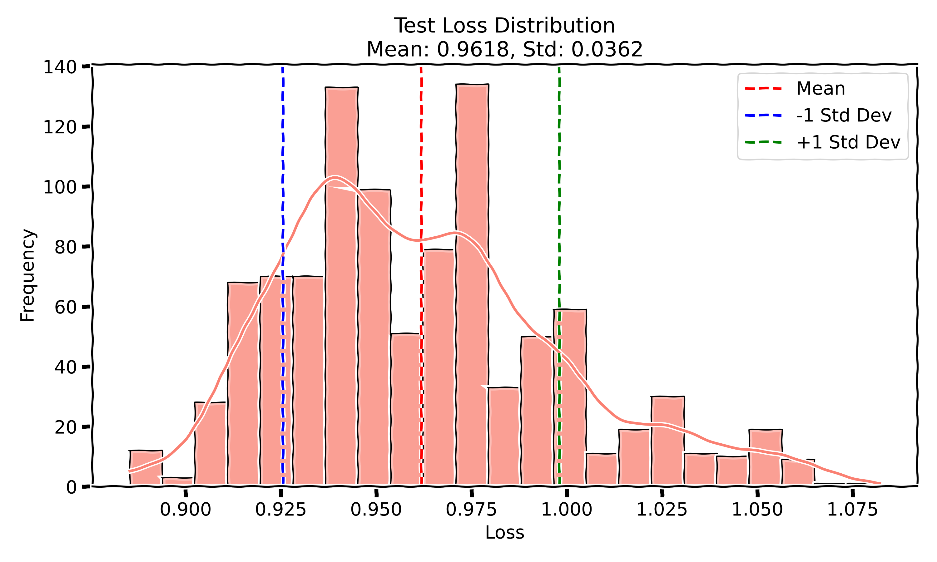
For this first setting, I wanted to leave things pretty standard, by allowing for both random initialization, and random shuffling of the training data into batches, training the model for 10 epochs, and then reporting/plotting the results on the test set, 1000 times, to visualize the variability.
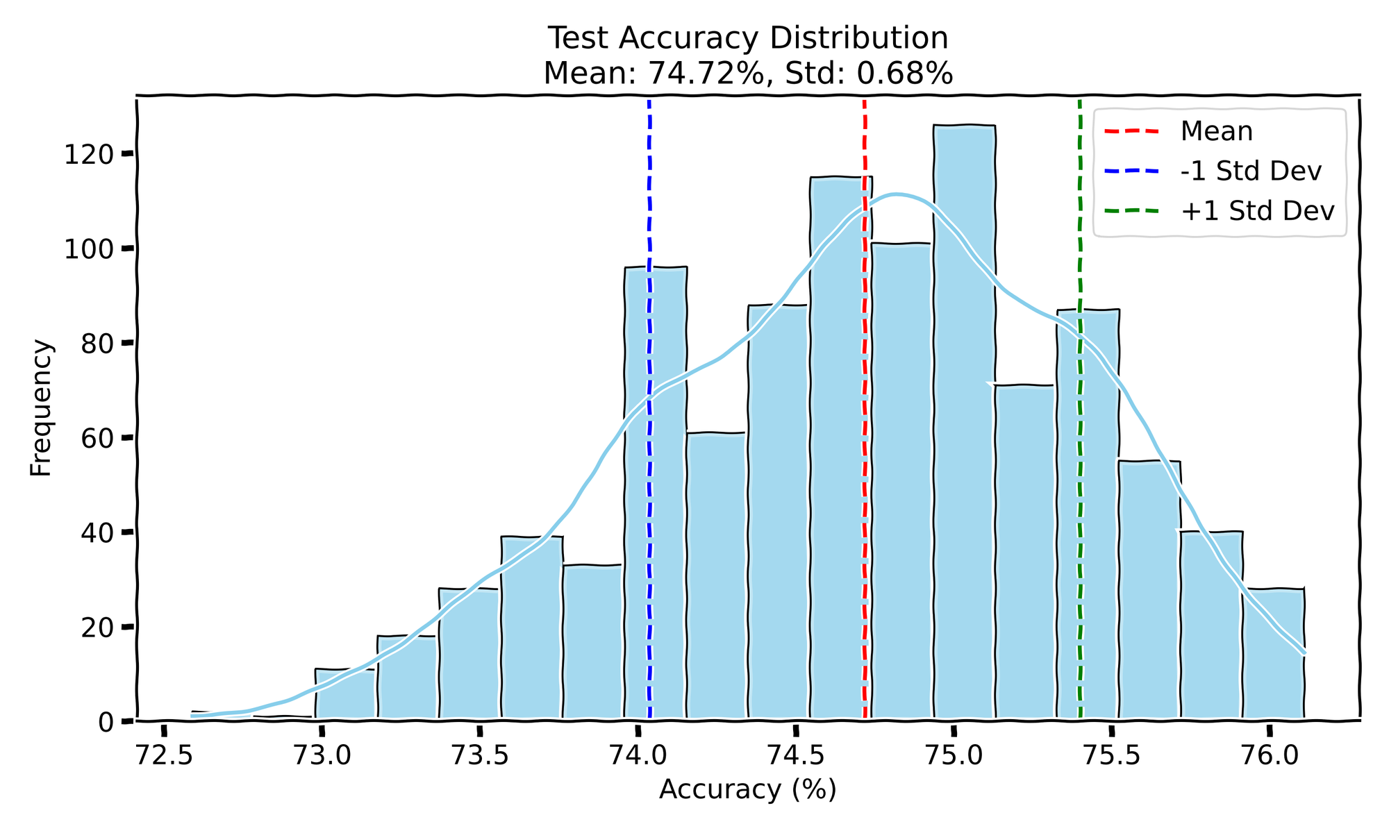
- Test Accuracy: The mean test accuracy is 74.72 with a standard deviation of 0.68.
- Test Loss: The mean test loss is 0.9618 with a standard deviation of 0.036.
Interestingly, the test loss appears to have a somewhat bimodal distribution, suggesting there might be two modes of convergence. In contrast, the test accuracy shows a single-mode Gaussian distribution, indicating that most runs converge to similar levels of accuracy. The training curves for both accuracy and loss are nearly on top of each other, showing little variability in the overall training process.
Experiment II
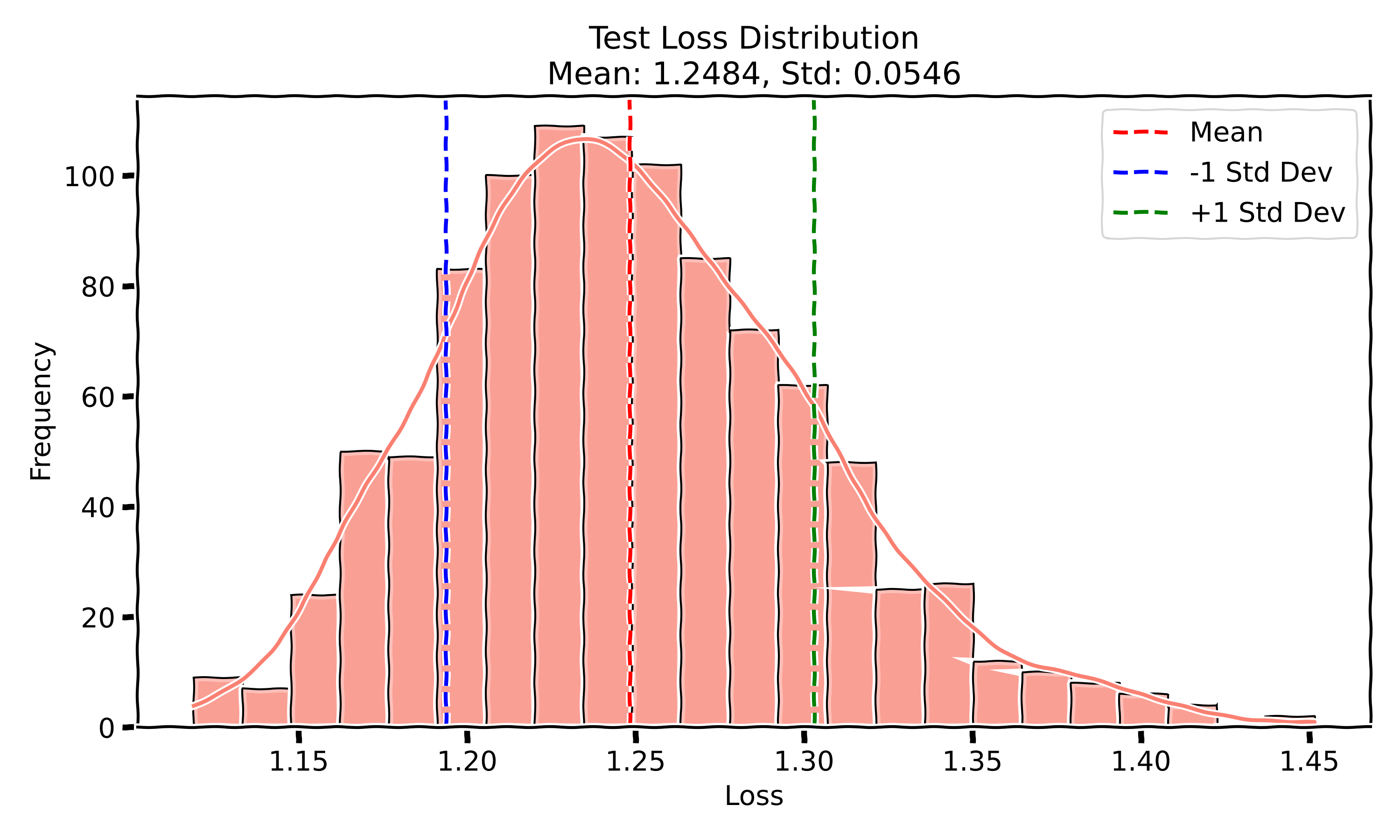
For the second experiment, I kept the data order fixed across all runs but allowed different random initializations for the network's weights. The idea was to see how much the variability in initialization alone would affect the outcomes. Here are the results for 1000 runs:
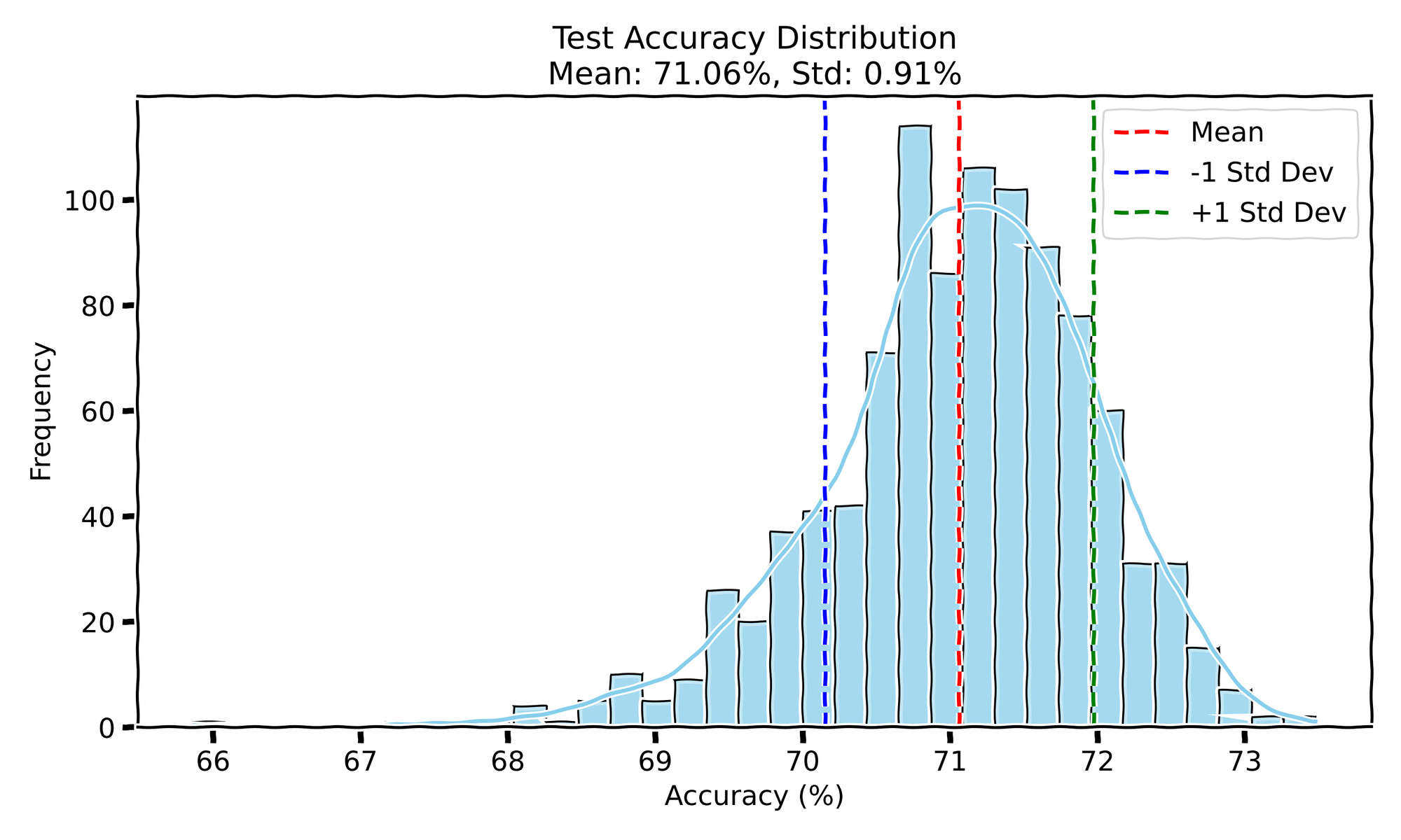
- Test Accuracy: The mean test accuracy is 71.06 with a standard deviation of 0.91.
- Test Loss: The mean test loss is 1.24 with a standard deviation of 0.0546.
This time, both the test accuracy and test loss display a single-mode Gaussian distribution, suggesting that varying the initialization of weights without changing the order of the data still leads to relatively consistent performance outcomes. The training curves remain closely aligned across all runs, indicating that initialization variability doesn't significantly affect training dynamics.
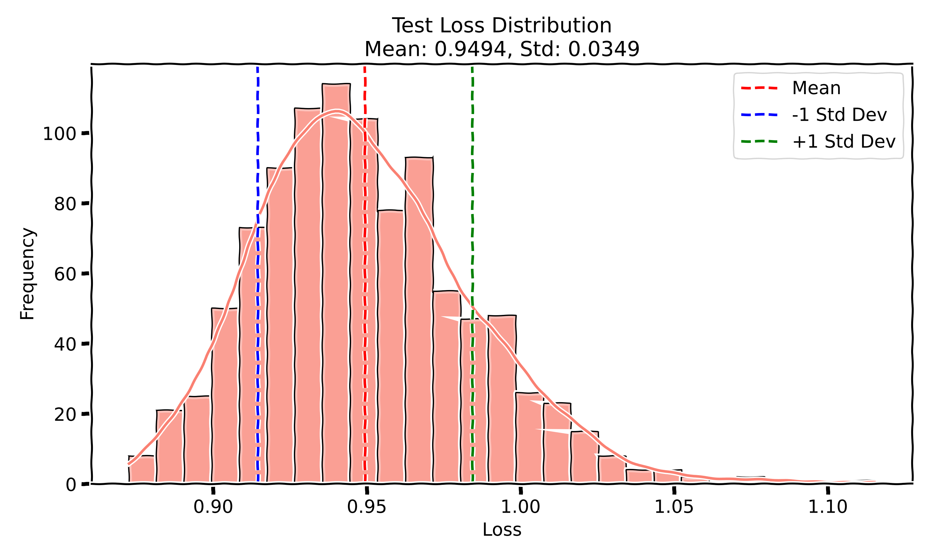
Experiment III
In the third experiment, I kept the network initialization the same for every run but shuffled the training data randomly for each run. This approach allows us to see how much of the variability in outcomes comes solely from the order of data presented during training, again for 1000 runs.
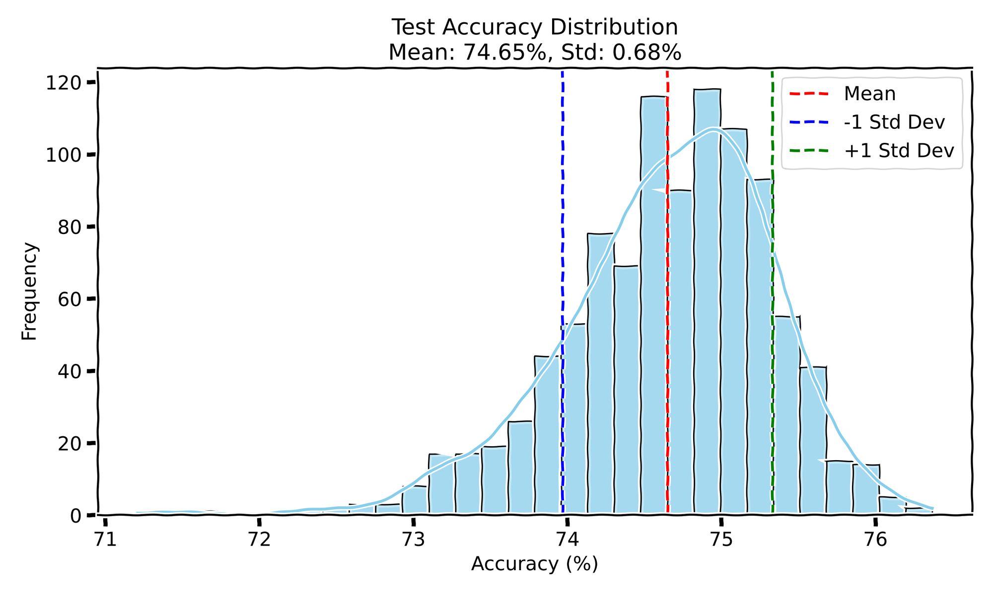
- Test Accuracy: The mean test accuracy is 74.65 with a standard deviation of 0.68.
- Test Loss: The mean test loss is 0.9494 with a standard deviation of 0.0349.
Like the first experiment, the test accuracy shows a single-mode Gaussian distribution, and the test loss is relatively tightly clustered. The training curves are, again, almost on top of each other, showing that even with different data orders, the model learns in a very similar manner each time.
Patterns in Variability
After running these experiments, a few patterns stand out when looking at the test accuracy and loss across the three setups. In Experiment I, where both initialization and data order were randomized, the model reached a mean test accuracy of 74.72% with a relatively small standard deviation of 0.68. The test loss showed a bit more variability with a mean of 0.9618 and a standard deviation of 0.036, with a slight bimodal distribution. This bimodal behavior in loss suggests the model may sometimes get stuck in a particular local minima during optimization, creating two different modes of convergence, while the accuracy stays more consistent. My guess is that this variance could be due to the combination of weight initialization and the order of mini-batch gradients, which occasionally drive the optimizer down a slightly worse valley.
In Experiment II, when I fixed the data order and only varied the initialization, the test accuracy dropped a bit to 71.06%, and the standard deviation increased slightly to 0.91. The test loss also saw a larger increase, hitting a mean of 1.24 with a slightly higher standard deviation of 0.0546. My take on this is that by fixing the data order, we removed a key source of randomness that helps the optimizer explore the loss landscape more effectively. Without that shuffle, the model might be more prone to getting stuck in suboptimal regions of the loss surface, explaining why the performance is a bit lower and more spread out.
In Experiment III, the results were similar to Experiment I, with randomized data order but fixed initialization, suggesting that the order in which data is presented during training has a larger influence on the model’s ability to converge to a good solution. The slightly higher test accuracy (closer to Experiment I) and the more consistent test loss reinforce the idea that data shuffling plays a big role in keeping the optimizer from getting stuck in bad local minima. Interestingly, the training curves across all experiments were quite close to each other, which implies that the model's training dynamics are pretty stable despite these random factors.
In both Experiment II and Experiment III, the accuracy distributions showed more pronounced heavy tails on the lower end, meaning there were more runs with significantly lower accuracy compared to Experiment I. This is particularly interesting because it suggests that reducing randomness, whether by fixing the data order or initialization, can occasionally lead to much poorer performance in some runs. It appears that without the combined randomness from both initialization and data shuffling, the model is more likely to get stuck in less optimal regions of the loss landscape, resulting in these occasional but notably poor outcomes.
So, what’s going on here? My hypothesis is that the interplay between data shuffling and random initialization helps the optimizer explore the loss landscape in a more diverse way, giving it more chances to find better generalizable solutions. When you remove or fix one of these sources of randomness, like in Experiment II, the optimizer’s exploration becomes more restricted, leading to slightly worse outcomes. The bimodal behavior in Experiment I’s test loss could be a sign that, with both randomness sources, the optimizer sometimes lands in a different region of the loss landscape.
Amplified Randomness
To push this even further, what if we intentionally introduced more controlled chaos into the system? One idea could be dynamically altering the data order during training—not just shuffling once per epoch but continuously reordering mini-batches based on certain criteria, like gradients or feature activations. Another approach might be to use more exotic initialization schemes where weight distributions aren’t just random but conditioned on some properties of the data itself, introducing a data-informed randomness right from the start. We could even experiment with periodically injecting noise into the gradients during backpropagation, forcing the optimizer to explore less-traveled regions of the loss landscape, kind of like a stochastic 'boost' to escape any suboptimal paths.
The point is, the randomness in neural networks is essential but also something we could actively tweak to nudge the network toward even more diverse and potentially better solutions. There’s room to experiment with pushing randomness in creative ways to uncover new optimization dynamics.
Final Thoughts
Overall, this was a small but interesting experiment, and while the results weren't exactly surprising, it was eye-opening to see how consistent the outcomes were across so many runs. It makes me reflect on the role randomness plays in training—something we often take for granted in machine learning. Can we harness or optimize this randomness in more meaningful ways? In the bigger picture, randomness isn’t just a byproduct of training—it’s a crucial part of how both artificial and biological intelligence handle the complexity of the world. It’s not just a tool, but a key ingredient that helps us learn, adapt, and find better solutions in unpredictable environments.
For the full code check out the GitHub repository.